1. 几何基础

1.1 点到直线的投影（垂足$\mathbf{P_F}$）

由于垂足在直线（经过点$\mathbf{P_0}$方向为$\mathbf{v}$）上，所以：
\[ \mathbf{P_F}=\mathbf{P_0}+\lambda\mathbf{v}\]
又由于垂直，则有：
\[ \begin{cases}
\mathbf{P_F}=\mathbf{P_0}+\lambda\mathbf{v}\\
(\mathbf{P_F-P_A})\cdot\mathbf{v}=0
\end{cases} \]
解得，
\[ \lambda=\frac{\mathbf{v}\cdot(\mathbf{P_A-P_0})}{||\mathbf{v}||^2} \]
所以（注意数量积的计算顺序），

\[
\begin{cases}
\mathbf{P_F}=\mathbf{P_0}+\lambda\mathbf{v}\\
(\mathbf{P_F-P_A})\cdot\mathbf{v}=0
\end{cases}
\]
解得，
\[
\lambda=\frac{\mathbf{v}\cdot(\mathbf{P_A-P_0})}{||\mathbf{v}||^2}
\]
所以（注意数量积的计算顺序），

\[
\mathbf{P_F}=\mathbf{P_0}+\mathbf{v}*\frac{\mathbf{v}\cdot(\mathbf{P_A-P_0})}{||\mathbf{v}||^2}
\]

• $*$：表示数乘，一般标量在前，矢量在后，但标量较复杂时也会反过来写
• $\cdot$：表示向量内积
• $\mathbf{v}^2$：表示内积的平方
• $v^2$：表示数量积的平方
• 下同

1.2 关于直线的对称点$\mathbf{P_S}$

利用上面点到直线投影的结论，可得推算出$\mathbf{P_A}$关于直线的对称点$\mathbf{P_S}$为：
\[
\begin{aligned}
\mathbf{P_S}=&\mathbf{P_A}+2(\mathbf{P_F}-\mathbf{P_A})\\
=&2\mathbf{P_F}-\mathbf{P_A}\\
=&2\mathbf{P_0}+2\mathbf{v}*\frac{\mathbf{v}\cdot(\mathbf{P_A-P_0})}{||\mathbf{v}||^2}-\mathbf{P_A}
\end{aligned}
\]

(*关于直线的对称点*)
fViewSymmetricPoint[pointView_, linePoint1_, linePoint2_] := Module[{
    pA = pointView,
    p0 = linePoint1,
    v = linePoint2 - linePoint1
    },
   2 p0 + 2 v (v.(pA - p0)/v.v) - pA
   ];

1.3 射线与平面的交点$\mathbf{Q}$

由于交点在射线（$\mathbf{P_A P_B}$）上，所以：
\[
\begin{aligned}
\mathbf{Q}=&\mathbf{P_A}+\lambda(\mathbf{P_B-P_A})\\
\lambda>&0
\end{aligned}
\]

由于交点在平面（过点$\mathbf{P_0}$，法向为$\mathbf{v}$）上，所以：
\[
(\mathbf{Q}-\mathbf{P_0})\cdot\mathbf{v}=0
\]

综上，
\[
\lambda=\frac{\mathbf{v}\cdot(\mathbf{P_0}-\mathbf{P_A})}{\mathbf{v}\cdot(\mathbf{P_B}-\mathbf{P_A})}
\]
当$\lambda<0$时，交点为射线的反向延长线与平面的交点
\[
\mathbf{Q}=\mathbf{P_A}+(\mathbf{P_B}-\mathbf{P_A})\frac{\mathbf{v}\cdot(\mathbf{P_0}-\mathbf{P_A})}{\mathbf{v}\cdot(\mathbf{P_B}-\mathbf{P_A})}
\]

(*射线与平面的交点*)
fRayPlane[rayPointA_, rayPointB_, planePoint_, 
   planeNormalDirection_] := Module[{
    pA = rayPointA,
    pB = rayPointB,
    p0 = planePoint,
    v = planeNormalDirection,
    k
    },
   k = v.(p0 - pA)/v.(pB - pA);
   If[k > 0,
    pA + k (pB - pA),
    None]
   ];

1.4 线段与球面的交点$\mathbf{Q}$

由于点$\mathbf{Q}$在半径为$R$球心为$\mathbf{C}$的球面上，所以：
\[
(\mathbf{Q-C})^2=R^2
\]

又由于点$\mathbf{Q}$在以$\mathbf{P_1}$（圆内）和$\mathbf{P_2}$（圆外）为端点的线段上，所以：
\[
\begin{aligned}
\mathbf{Q}=&\mathbf{P_1}+\lambda(\mathbf{P_2-P_1})\\
\lambda\in&[0,1]
\end{aligned}
\]

将线段方程代入球的方程：
\[[\mathbf{P_1}+\lambda(\mathbf{P_2-P_1})-\mathbf{C}]^2=R^2\]

\[(\mathbf{P_2-P_1})^2\lambda^2+2(\mathbf{P_2-p_1})\cdot(\mathbf{P_1}-\mathbf{C})\lambda+(\mathbf{P_1}-\mathbf{C})^2-R^2=0\]

根据一元二次方程求根公式，计算$\lambda$（注意数量积的计算顺序）
\[
\lambda=\frac{-(\mathbf{P_2-P_1})\cdot(\mathbf{P_1}-\mathbf{C})\pm\sqrt{[(\mathbf{P_2-P_1})\cdot(\mathbf{P_1}-\mathbf{C})]^2-(\mathbf{P_2-P_1})^2[(\mathbf{P_1}-\mathbf{C})^2-R^2]}}{(\mathbf{P_2-P_1})^2}
\]
由于，$\lambda<0$时，为$\mathbf{P_2}\mathbf{P_1}$延长线上的点，
所以要求的交点为：
\[
\mathbf{Q}=\mathbf{P_1}+(\mathbf{P_2-P_1})*\frac{-(\mathbf{P_2-P_1})\cdot(\mathbf{P_1}-\mathbf{C})+\sqrt{[(\mathbf{P_2-P_1})\cdot(\mathbf{P_1}-\mathbf{C})]^2-(\mathbf{P_2-P_1})^2[(\mathbf{P_1}-\mathbf{C})^2-R^2]}}{(\mathbf{P_2-P_1})^2}
\]

(*射线与球的交点*)
fRaySphereItsc[pointInSphere_, pointView_, sphereCenter_, 
   sphereRadius_] := Module[{
    p1 = pointInSphere,
    p2 = pointView,
    c = sphereCenter,
    r = sphereRadius,
    k, k1, k2},
   k1 = -(p2 - p1).(p1 - c);
   k2 = Sqrt[k1^2 - (p2 - p1).(p2 - p1) ((p1 - c).(p1 - c) - r^2)];
   k = (k1 + k2)/(p2 - p1).(p2 - p1);
   If[k2 \[Element] Reals && k > 0,
    p1 + k (p2 - p1),
    None]
   ];

1.5 旋转+平移变换（绕x轴旋转$\theta$后，沿$z$轴平移$d$）

\[
\left(
\begin{array}{cccc}
1 & 0 & 0 & 0 \\
0 & \cos (\theta ) & -\sin (\theta ) & 0 \\
0 & \sin (\theta ) & \cos (\theta ) & d \\
0 & 0 & 0 & 1 \\
\end{array}
\right)
\]

(*从向量{x1,y1,z1}旋转到向量{x2,y2,z2}*)
RotationTransform[{{x1,y1,z1}, {x2,y2,z2}}]

2. 怎样用 Mathematica 实现

2.1 基本思路

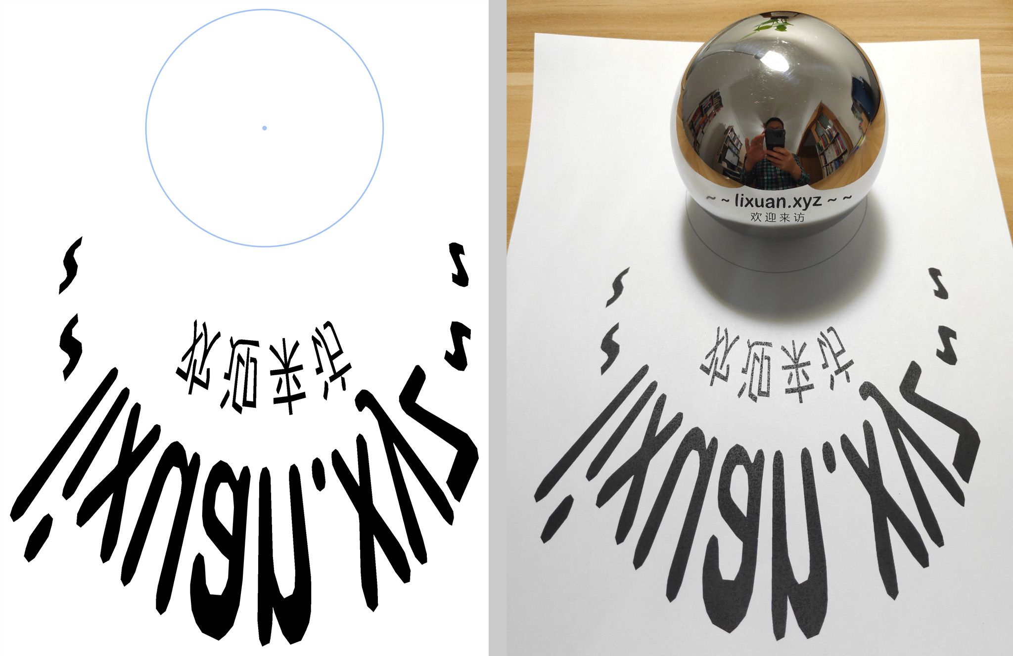
为简单起见，只考虑二值图像的球面反射成像。
即便没有上面的几何知识，用Mathematica也可以非常方便的实现，详见文章——“Anamorphic Reflections in a Christmas Ball-YOZ”。
不过，使用上面的几何知识，可以让计算速度更快。

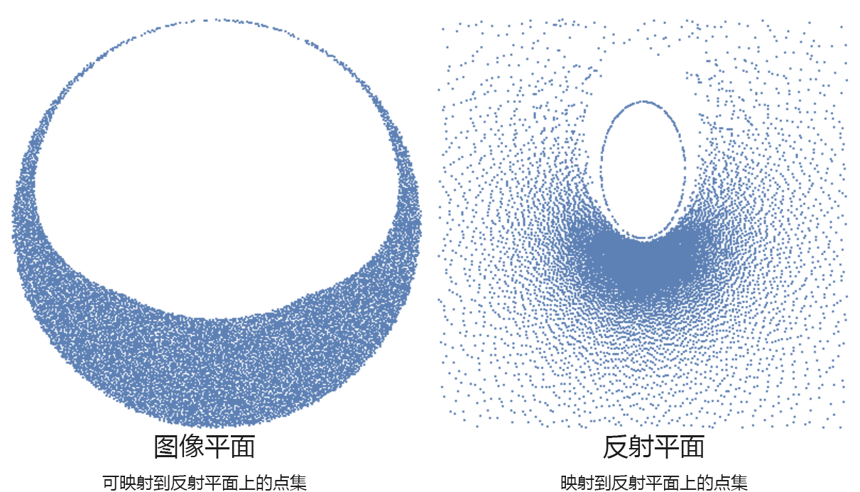
1. 将二值图像转为“区域 – Region”，并提取边界坐标（这样做不但可以减少计算量，还可以输出矢量图）
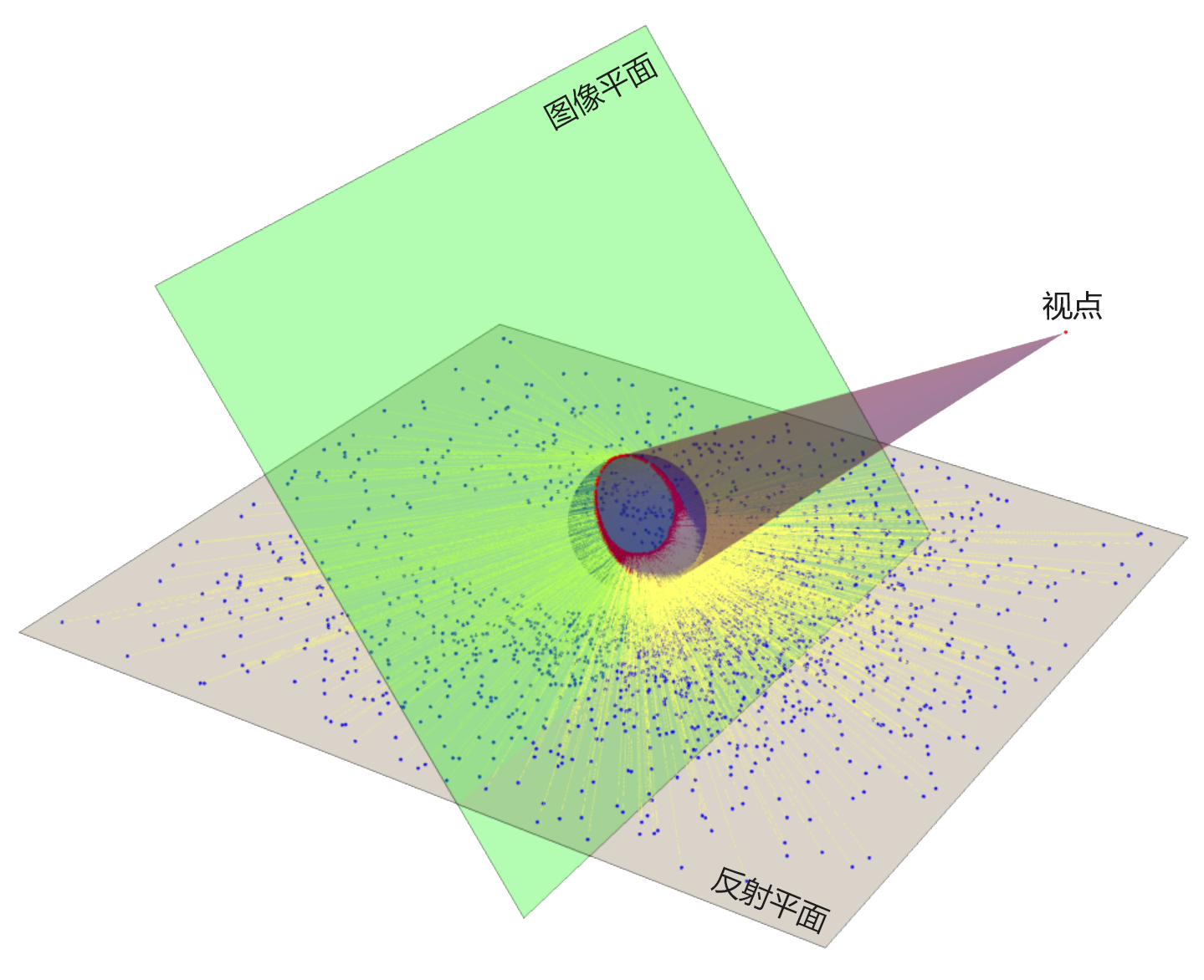
2. 将边界坐标三维化，并旋转到“图像平面”，并进行缩放（缩放需要计算很多点，但一般只计算一次即可）
3. 将图像平面上的坐标映射到反射平面
4. 将坐标转换为“区域”，并绘图

2.2 缩放

(*================ 计算缩放 ================*)
{w, h} = Flatten[
   Differences /@ 
    CoordinateBounds@MeshCoordinates[regionImage]];(*输入图像内容的宽高*)
maxCellMeasure = 0.2;
imagePoints2D = 
  MeshCoordinates@
   DiscretizeRegion[
    Disk[{0, 0}, Sqrt[cSphereRadius^2 - Norm[imageCenter]^2]], 
    MaxCellMeasure -> {"Length" -> maxCellMeasure}];(*2维圆盘上的点*)
imagePoints3D = 
  RotationTransform[{{0.0, 0.0, 1.0}, 
     cViewPoint}][#~Join~{Norm[imageCenter]} & /@ 
    imagePoints2D];(*3维视觉平面上的点*)

pointsT = fViewPointToReflectPoint /@ imagePoints3D;(*3维反射平面上的点*)
pointsPairNew = 
  Select[pointsT, #[[2]] =!= None && #[[2]] \[Element] Reals && 
     Max[Abs[#]] < 30 &];(*简单筛选*)
pointsImage2D = (RotationTransform[{cViewPoint, {.0, .0, 1.0}}]@
     pointsPairNew[[;; , 1]])[[;; , ;; 2]];(*旋转回2维平面*)

yMax = Select[pointsImage2D, Abs[#[[1]]] < 0.1 && #[[2]] < 0 &][[;; , 
     2]] // Max;
{xMax, yMin} = 
  SortBy[Select[pointsImage2D, 
     Abs[(#[[2]] - yMax)/#[[1]]] < h/(w/2) && #[[2]] < yMax &], 
    Last][[1]];
xMax = Abs[xMax];

imageNewRange = {{-xMax, xMax}, {yMin, 
    yMax}};(*将图像缩放到图像平面上的该区域：{{xMin,xMax},{yMin,yMax}}，\[FilledSquare]\
\[FilledSquare]y可适当调大\[FilledSquare]\[FilledSquare]*)

2.3 完整代码下载

修改图中黄色方框中的文字，逐步运行即可生成自己想要的结果 ^_^